Overview
We trained a 2D convolutional neural network with an optimised topology in order to perform multiclass classification on image data. The images represent spatiotemporal representations of strain disturbances on a subsea fibre optic cable as measured by distributed acoustic sensing (DAS) technology.
The cable was installed on the ocean floor close to the Nankai Subduction Zone offshore Cape Muroto, which recorded seismic activity across its 50km length for several months. Within this seismogenic zone, where slow-slip (SSEs) and very-low frequency earthquakes (VLFEs) are common, a range of different hydroacoustic signals were clearly indicated on the DAS images.
Enhancing monitoring capability for fibre optic seismology
As Figure 1 shows, each recorded DAS waveform (a total of more than 10,000 channels synchronised together) is firstly bandpass filtered (and further pre-processed) in order to reveal the seismic activity, before being converted into an image. Traditionally, the cataloguing of events is being done by an expert seismologist.
Given the huge amount of data generated by DAS (close to 1TB per day) and the associated high probability of human error in detecting seismic events in a manual way, a more efficient and automated alternative has been developed. In particular, a classification model is now used to replace the human-in-the-loop process by automatically cataloguing these events and producing a report of probabilities per event detected. That is, the probability whether an event is an earthquake given the training data inputs P(geophysical | inputs).
The stakeholders (JAMSTEC researchers) agreed that the top priority for them would be a system able to discriminate between geophysical and non-geophysical events and this has been implemented in view of further extending it during future research activity.
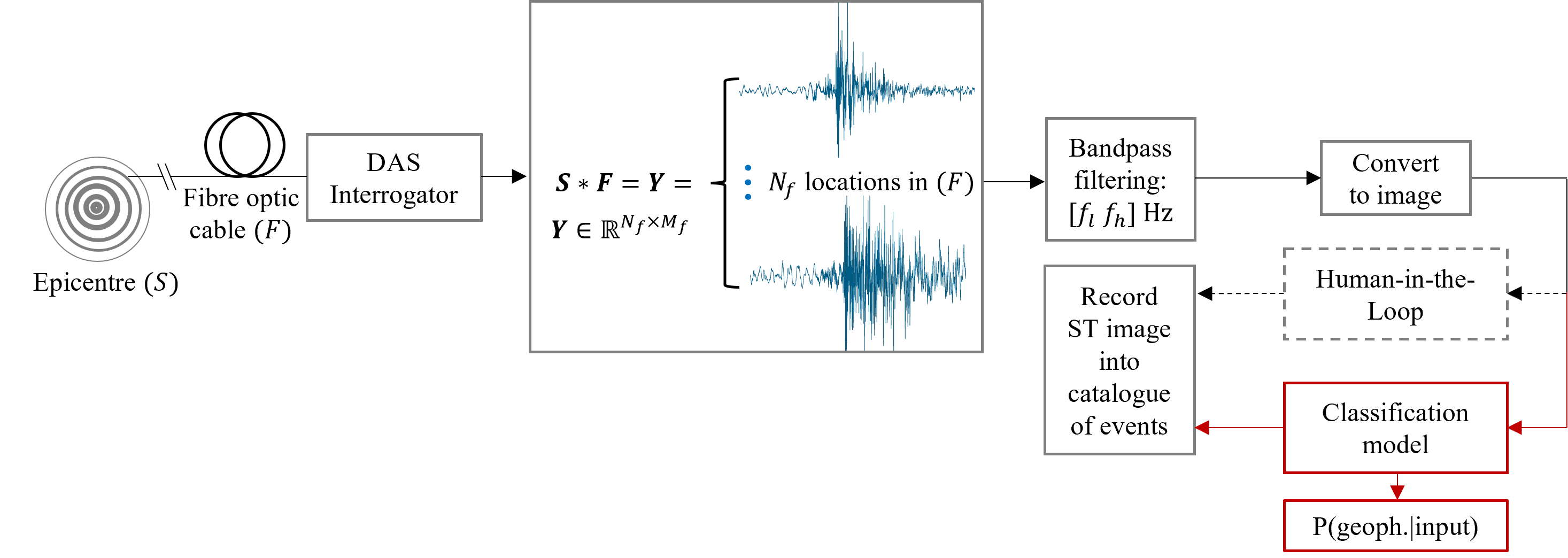
Figure 1. Overview of image acquisition and earthquake cataloguing process.
Classification model specifics and main results
On a test set of more than 100 images, our classifier yields a classification accuracy of more than 90%. One of the major issues that we faced while training our classifier was the fact that our available training dataset was relatively small, e.g. around 800 images for all three classes. This significantly challenges the generalisation performance of any type of neural network trained on images with complex patterns and shapes. We addressed this issue by employing a Bayesian Optimisation approach, which is typically solved using a surrogate model, e.g. one based on Gaussian Processes regression, which serves as a proxy to the original objective function.
The optimised hyperparameters (given a feasible search space of values) include: the number of 2D convolutional kernels in each layer, the depth of the network (number of layers), the nonlinear activation function and the addition of layers such as batch normalisation and dropouts. In particular, dropout layers proved to be an important feature for our neural network topology since they help prevent overfitting the network on the training images (and therefore, can train for longer). Dropout layers were included after each 2D convolutional layer in the network.
We optimised most of the hyperparameters using Keras Tuner with more than 35 trials. After this process, validation accuracy climbed very close to 98% for several hypertuned topologies we tested. As an example, in Figure 2 we show the two-dimensional contour plots (interpolated values) of 4 different hyperparameters during their optimisation process.
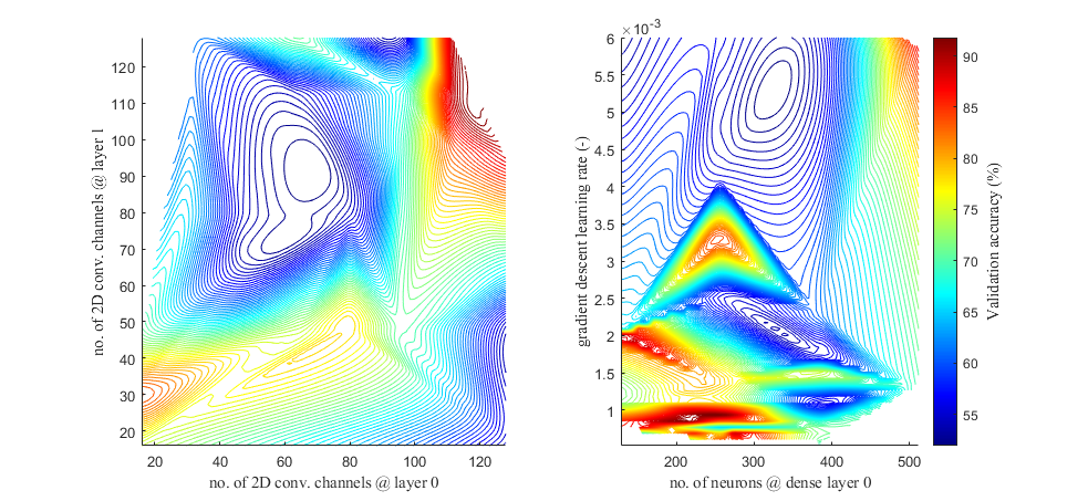
Figure 2. Two-dimensional contour plots showing an example of hyperparameter tuning: Optimisation of the number of 2D convolutional channels at network layer 0 and 1 (left image). Optimisation of the number of neurons at fully connected dense layer 0 and gradient descent learning rate (right image).
As an example, the variation in the loss function and classification accuracy on the validation set during the training phase of two hyperparameter optimised models (Bayes and Bayes-IA) and a non-hyperparameter optimised model (Base) is shown in Figure 3. Note that Bayes-IA is a classifier with an extra set images added on its training set after random pre-processing them (random changes in brightness and contrast levels, random cropping and zooming, etc.).
Both hyperaparameter-optimised models achieved classification accuracies close to 95%. On the other hand, the Base model achieved 90%.
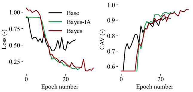
Figure 3. Variation in validation accuracy of loss function (left) and classification accuracy (right) for three different classification models.
What is most important, however, it is the accuracy on the test set. In Figure 4 the confusion matrix of all three classes for the three different models is shown. In particular, Bayes achieves the highest overall test accuracy.
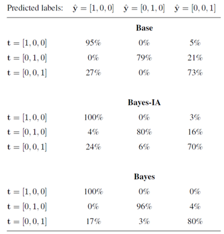 Figure 4. Confusion matrix on a test set. Geophysical class is t=[1,0,0], Ambient Noise is t=[0,1,0] and Non-geophysical class is t=[0,0,1].
It should also be noted that the hyperparameter optimisation phase took approximately 2 hours on a single NVIDIA V100 with 256 x 256 grayscale input images.
Conclusions and future research directions
As the results demonstrate, the trained classifier model with an optimised choice of hyperparameters is robust and effective in classifying low signal-to-noise ratio (SNR) DAS dynamic strain data arising from multiple sources of hydroacoustic energy.
An incremental approach (i.e. addition of further classes to the classifier) has recently been devised.
Additionally, the detection of earthquakes without apriori knowledge or data availability of such events is currently being explored. That is, we consider a model that detects anomalies, i.e. anything that is not ambient noise or non-seismic event. Among other benefits such as the immediate deployment for monitoring anomalies, it has the added benefit that it can detect rare and never seen before events.
Some further details regarding 2D convolutional neural networks
Convolutional neural networks typically comprise of the following main components: 2D convolutional layers, non-linear activation functions, 2D pooling layers and fully connected dense layers, as shown in Figure 4. The purpose of adding 2D convolutional layers (b)(d)(g)(i)(k), is both to extract useful features and to minimise the number of parameters to be optimised. This is especially important in complex image discrimination tasks, where there are very subtle patterns to learn from each class. This necessitates the learning of a suitable set of 2D filters, i.e. 2D convolutional layers, that maximise the discrimination accuracy between sets of classes. As shown in Figure 4, an input image (a) is convolved with a large set of 2D filters (b), whose parameters are optimised as part of the network. The results of the convolution operations, at the earlier depths of the network, result in the extraction of simple image features (c), such as edges and corners. Although this can be, relatively easily achieved with a well-designed set of filters, e.g. Laplacian edge detectors, at greater layer depths, e.g. (f)(j)(l), it is not clear how one may design/select classical filters to extract more abstract-level features. The strength of the classification model lies on the fact that we can learn these filters, as part of the network, while at the same time their weight-sharing properties enable one to reduce the exponential rise of network parameters, which is a typical characteristic of feedforward neural networks (m)-(p).
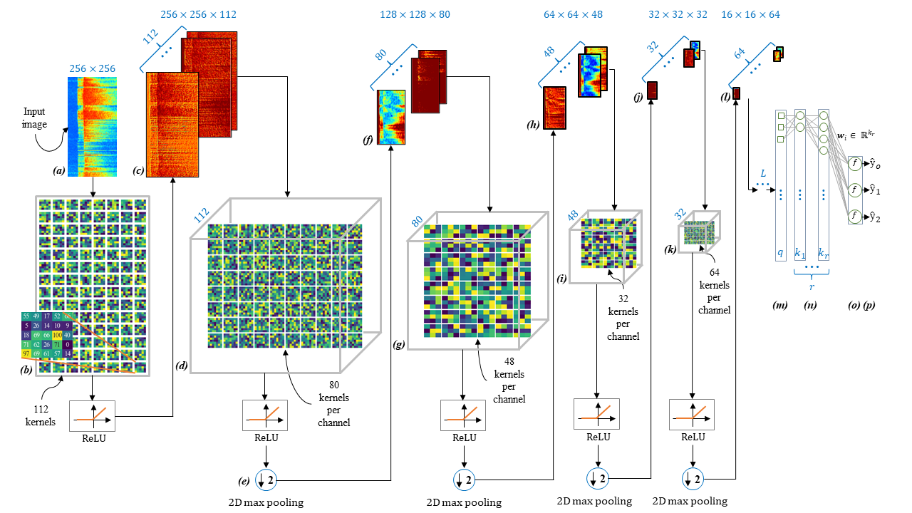
Figure 4. Diagram of the CNN model, illustrating some of its main components, including 2D convolutional and pooling layers.
